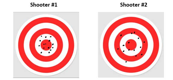
Consider the follow two targets:

Shooter #1 and Shooter #2 both fired 15 rounds into their respective targets. Who is the better marksman?
Most people would agree that Shooter #1 is better since all 15 of his rounds are grouped within the inner two rings. Shooter #2 is pretty good, but many of his shots landed in the third ring; one even landed in the fourth ring. Since minimizing variation from the center bullseye is the object in target shooting, and Shooter #1 demonstrated the lesser variation of the two shooters, then Shooter #1 is the better marksman. Right?
Maybe not. Before we decide who’s the better shooter, let me add one more detail to the puzzle:
Shooter #1 was positioned 10 meters away from the target, and Shooter #2 was positioned 1,000 meters from the target. Now who is the better marksman?
Examples like this reveal an important phenomenon: all else equal, the variation within a dataset is dependent on the magnitude of its mean. And a statistical tool called the Coefficient of Variation (CV) helps us compare the variation of datasets when the magnitude of the things we’re measuring is different.
Let’s consider a hypothetical example from the animal world:
Imagine we weighed 100 Cairo Spiny Mice and 100 African Bush Elephants, and then analyzed the data. We might find something like this:

Well, it’s certainly no surprise that the standard deviation of the elephant weights is massively larger than that of the mice. The world would be a much scarier if this weren’t true!
But the question to ask when comparing creatures (or processes) of different sizes is not “How do their standard deviations compare?”, but “How do their relative standard deviations compare?” And this is where the simple, yet effective Coefficient of Variation really shines. Let’s consider the equation:
CV = (Standard Deviation / Mean) * 100
This formula allows you to examine the variation of your data relative to its mean. Using our study of mice and elephants, we find:
CVmice = (3.20 / 42.61) * 100 = 7.51%
CVelephants = (395 / 5910) * 100 = 6.68%
So, while it’s obvious that the expected weight range of mice is less than that of elephants, it may be a surprise that their relative weight distribution is actually greater.
CV also offers its users a more useful way to express standard deviation. Instead of a stand-alone number like 3.20 grams, we can now express it as a percentage of the mean, giving the parameter some needed context.
The applications of CV are plentiful. In finance, CV is used to measure the volatility of a stock’s price. In medicine, CV is used to measure shifts in a patient’s test results. And in manufacturing, CV is used to compare closely related processes. For instance, imagine a saw cutting operation in a factory that manufacturers threaded pipe. The same saw may cut a wide variety of pipe diameters and lengths. A quality engineer could use CV to compare the saw’s capability across a range of cut lengths.
For a deep dive into using statistics like CV to monitor and analyze your manufacturing process, check out the online course titled, “Process Capability Analysis”, and other resources at themanufacturingacademy.com.

