by
Mark Fiedeldey and Ray Harkins
Business today is more competitive than ever. As a result, successful business leaders often need to make quick decisions with less than complete data. The wrong decision could result in significant losses, layoffs, or worse. This is where quality professionals and other data-savvy specialists can offer some assistance: by making the best analysis possible given the available data.
Without a deeper understanding of analytics, most managers make their projections based on single-point estimates like average revenue, average cost, average defect rate, etc. After all, the arithmetic average of any of these values is generally considered the best guess to use for projections. But complex decisions with broad potential consequences deserve more than “back of the napkins” estimates. They require the use of all available data, not just their averages.
Consider the following case study:
Monster Machines, a manufacturer of custom off-road vehicles, began purchasing axles six months ago from Axles “R” Us. But Axles “R” Us has struggled to meet their production demand, resulting in Monster sourcing additional axles from A1 Axle four months ago. However, the quality coming from A1 Axle has been lower than expected. As a result, Monster’s quality manager, Mike Rometer, is wondering whether an investment in additional workstations at Axles “R” Us, which would allow them to meet the full production demand, is a good decision for Monster.
Given the various costs and savings associated with sourcing axles from a single supplier, Monster’s CFO, Penelope Pincher, estimates that a monthly savings of $750 on incoming quality is needed to justify the elimination of A1 Axle. Mike needs to determine if Monster could save $750 per month by sole-sourcing the axles from Axles “R” Us.
He tallied the monthly incoming quality cost records for both suppliers with the following results:
Table 1. Monthly Incoming Quality Cost ($)

Since historical records showed no seasonality with the production of the vehicles, the simplest comparison Mike can perform is to examine their average monthly quality costs. The average monthly cost for Axles “R” Us is $2,206.95, and the average monthly cost for A1 Axle is $3,231.74.
With Monster’s proposed investment, Axles “R” Us will be able to meet the production demand without the need for a second supplier. Axles “R” Us has also guaranteed their quality costs will not increase even with the added production. Thus, Monster’s proposed investment coupled with Axles “R” Us’s quality commitment results in an average quality cost savings of $1,024.79 per month. This is well above Penelope’s threshold of $750 per month, and therefore looks like the obvious choice.
However, each supplier’s average quality cost is a mere single point estimate of their incoming quality. While a valid estimate, the arithmetic average isn’t complete enough for use in critical decisions as it ignores any variation in the data.
Mike then decided to perform a more in-depth analysis of the quality data beginning with determining its underlying probability distribution. While random variables can often be modeled as normally distributed, more detailed analyses require verification of the underlying probability distribution before proceeding.
To better understand the spread of the cost data over time, Mike started his new level of analysis by first calculating the standard deviation of his quality cost data for both suppliers. The standard deviations were $166.99 and $117.44 for Axles “R” Us and A1 Axle, respectively. He then used the Shapiro-Wilk1 statistical test on their data, which allowed him to infer that in fact their quality costs could be modeled with a normal distribution.
With the arithmetic average and standard deviation for each, he then subtracted Axles “R” Us’s distribution of cost data from A1 Axle’s distribution of cost data, resulting in a new normal distribution of monthly savings data.
Subtracting normal distributions involves two steps for non-correlated variables like these:
First, subtract the means to derive the mean of the resulting normal distribution. And second, take the square root of the sum of the squared standard deviations to derive the standard deviation of the resulting normal distribution. When Mike stepped through this process on his cost data, he arrived at the following:
Table 2. Distribution of Savings
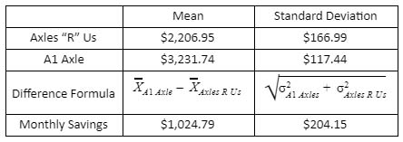
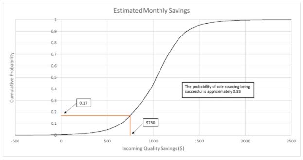
Monster’s monthly savings distribution has an average of $1,024.79 and a standard deviation of $204.15. Entering these new distribution parameters into Excel’s norm.dist formula2, Mike estimated that the probability of saving at least $750 is about 0.91. He also generated the chart below showing the cumulative estimated monthly savings distribution:
Figure 1: Estimated Monthly Savings
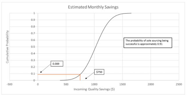
Mike’s analysis showed the staff at Monster that single-sourcing their axles from Axles “R” Us is likely to save them more than $750 per month, but it’s not the sure bet suggested by his analysis using the averages only. Understanding that their risk of failing to exceed the $750 threshold is about 9% may influence their decision.
Mike knew that his second analysis, while intricate, utilized more of the available data and offered an estimation of risk not attainable by simply examining averages. But he also knew that this second analysis also depended on the accuracy of each supplier’s distribution parameters. After all, repeated sampling to estimate these same parameters would generate slightly different results each time.
In fact, random variables can be modeled with an infinite number of normal distributions, each with a slightly different set of parameters. Some models would be better fitting than others, but there is no way to determine which pair of parameters, if any, describe the “true” distribution.
These various pairs of possible parameters form their own distribution—a joint probability distribution—that analysts can use to account for uncertainty in the parameter estimates.
Unlike common probability distributions like Normal and Exponential that have equations to describe them, there is no equation to describe this joint probability distribution of parameters. The only option is to use numerical techniques to generate a sample of the distribution. With sufficient samples in a numerically generated estimate, the uncertainty in the parameters can be adequately estimated.
One class of algorithms called the Markov Chain Monte Carlo (MCMC) method is commonly used for this purpose. The specific algorithm used in this example is called the Metropolis-Hastings.3
When our quality manager Mike applied this MCMC method to the incoming quality cost data of the Axles “R” Us and A1 Axle data, he generated the joint mean/standard deviation distributions Figures 2 and 3, respectively. Each distribution was based on 750,000 samples.
Figure 2: Axles “R” Us
Joint Distribution of Normal Parameter Pairs
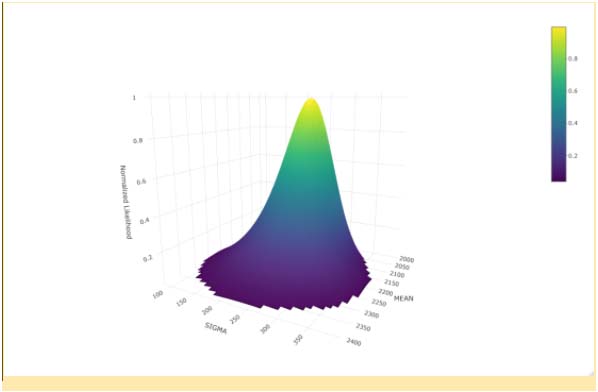
Figure 3: A1 Axle
Joint Distribution of Normal Parameter Pairs
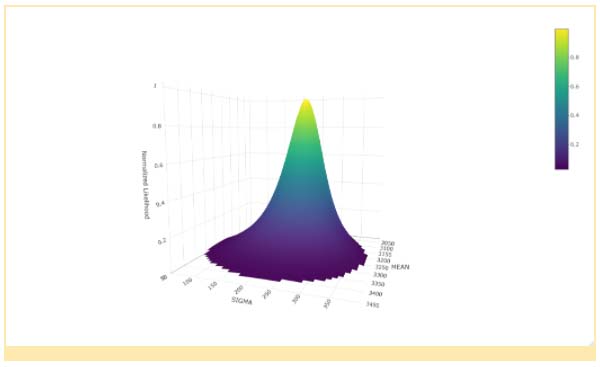
The first detail to note in these estimated joint probability distributions is that the single point estimates of the parameters, namely mean and standard deviation, are right in the heart of the MCMC sampled distribution. This should make Mike feel confident his earlier analysis was valid.
The second interesting detail is the range of possible pairs of parameters that could model the cost data. For example, normal distributions with means between $2,000 and $2,400 and standard deviations between $100 and $400 appear from the graphics to be useful model contenders for the Axles “R” Us data. Perhaps the wide range is primarily a consequence of having only six data points. But the fact remains that the uncertainty in these parameters is quite large. To reduce this range of values, Mike may choose to postpone his decision to single source axles until they can collect more data. Nonetheless, this is the best summary he can provide given the current data.
Based on this joint probability distribution for each supplier, Monster can estimate the future monthly incoming quality cost distribution for each supplier in a manner that includes the uncertainty in the distribution parameters. The monthly cost difference between the two suppliers can then be simulated and the savings estimated. The predictive distribution of simulated monthly savings, based on 25,000 simulated monthly costs, is shown in Figure 4.
Figure 4: Estimated Predictive Monthly Savings
Accounting for Parameter Uncertainty
Mike’s newest analysis, accounting for the uncertainty in each supplier’s cost distribution parameters, raised the risk of not meeting the threshold of $750 monthly savings from 9% to 17%–a significant enough shift to potentially influence their decision.
This case study illustrates that basing decisions on analyses using point parameter estimates ignores significant sources of uncertainty, potentially resulted in bad decisions. The first analysis, which was a point estimate average accounting for no uncertainty, suggested sole sourcing to Axles “R” Us was an absolute win. The second analysis, which accounted for uncertainty in monthly incoming quality costs but used point estimate parameter values, suggested a risk of failure of about 9%. And the final analysis, which accounted for both the uncertainty in monthly costs as well as the uncertainty in the distributional parameter values, raised the risk of failure to about 17%.
In an actual quality-related case familiar to the authors, engineers were asked to examine capability data from a forging process using a similar analytical approach. A manufacturer was hot forging the rough shape used to make the inner rings for an automotive wheel bearing. The forged rings were then CNC turned to form its final shape used in the bearing assembly. Therefore, the dimensions of the forged components were critical to the subsequent turning process. Too much material on the forged components resulted in premature tool wear in the turning process. Too little material resulted in “non clean up” surface defects on the final part.
Thirty samples of the forged ring were randomly drawn from an initial production run of 500 pieces. The overall width of these samples was measured on a CMM and the data was analyzed with the following results:
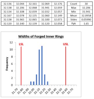
The engineering specification for the width was 32.200 +/- .400 millimeters. Using the standard capability index formula,
![]()
results in a Ppk of 1.65. Observing the histogram, we see that the data is slightly shifted toward the lower specification limit. Using the Microsoft Excel formula,
NORM.DIST (x, mean, standard deviation, cumulative)
we find that the expected parts per million below the lower spec limit equals .39.
These results, like the earlier supplier quality cost example, are based on single-point estimates of the process distribution and the assumption that the future production will produce parts with the exact same distribution parameters. Ignoring the inherent uncertainty of these parameters and assuming the future is as certain as the past builds into our conclusions an optimistic bias.
Given that historical data has shown that the manufacturing equipment used to produce parts similar to these has variation that is well modelled with a Normal distribution, we can use the same MCMC technique employed for the Monster Machines example above to estimate the individual and joint distributions of the parameters. The results are shown below.
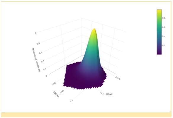
Note that the mean of our 30-piece sample measurements is nearly identical to the mode of the MCMC distribution of means. Likewise, the standard deviation of the 30-piece sample data is nearly equal to the mode of the MCMC distribution of standard deviations.
The parameter distributions shown above represent the parameter values for a Normal distribution from which the sample data is likely to have been derived. So, the single-point estimates found in Excel are not necessarily wrong. They are just one of many potential sets of parameters for the underlying distribution. Since there is no way to know the true parameter values, we can instead utilize all potential parameter sets that are likely to be true to generate our results.
Using these parameter distributions, we can generate an estimate for the distribution of future production. The cumulative distribution function (CDF) of that predictive distribution is shown below.

From the predictive CDF, a large sample of measurements is drawn and used to calculate the mean, standard deviation, resulting future capability index, and PPM defective.
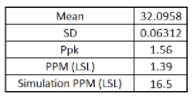
The Ppk found in Excel was 1.65. The Ppk for future production found by considering model parameter uncertainty as 1.56. The simulated PPM defective is about 17 as compared with the Excel result of 0.39. The risk of producing 17 PPM defective may be sufficient to investigate the process and implement actions to reduce this risk.
Whether or not the manufacturing process is deemed qualified is not the decision of the analyst. The role of the analyst is to provide results using the best techniques available, and as we have seen, single point estimates ignore the inherent uncertainty in distributional parameters.
As quality engineers and data analysts, decision makers often look to us to capture and crunch the data available to make major decisions. Analytical tools like MCMC allow us to extract far more insights than we could with the simpler, single-point estimate techniques.
Footnotes:
- The Shapiro-Wilk test for normality used was an Excel add-in function SWTEST(data,original,linear) downloaded free from Charles Zaiontz’ website: https://www.real-statistics.com/tests-normality-and-symmetry/statistical-tests-normality-symmetry/shapiro-wilk-test/
- =1-norm.dist(threshold, average, standard deviation, Cumulative Yes or No)
- The R code for the Metropolis-Hastings algorithm was downloaded free from Mark Powell at his consulting website https://www.attwaterconsulting.com/ and then modified for this case study. The R programming language (also free to download) has a package called MHadaptive which includes a function called Metro-Hastings