Several years ago, I was trying to fill a quality engineer’s position within my department. One person’s resume caught my attention. Under a section titled “Areas of Expertise”, it read “Quality Engineering Statistics”. “My gosh”, I thought, “We’ve got to call this guy for an interview.”
A week later, I sat across the conference table from this gentleman as we talked about his experience and career goals. Wanting to a bit more dig into his analytical skills, I asked “What’s the difference between Cpk and Ppk?” Immediately the blood drained from his face. I thought perhaps the ghost of one of his dead relatives walk in the room. But I looked around and didn’t see any apparitions. After an awkwardly long pause, he responded, “Isn’t one of them short term and the other one long term?” Even though I courteously continued our conversation for several more minutes, the interview was over at that moment.
Setting aside the problem of people embellishing resume details, this conversation started my realization about the significant block of quality professionals who can’t explain the differences between these two common capability indices. (If you haven’t yet read the first article in this series titled, “What is Process Capability Analysis? Really.”, you may want to read it first to pick up the fundamentals on these indices.)
The easiest way to begin understanding the difference between Cpk and Ppk, and their corollaries Cp and Pp, is to look at their formulas:

Quickly we can spot that the numerators for Cpk and Ppk are identical as are the numerators for Cp and Pp. In fact, the only difference between these formulas is the use of sigma-hat in the denominators of Cp and Cpk, but sigma in the denominators of Pp and Ppk.1 Sigma is the Greek letter often used in statistics to represent the sample standard deviation, a common measure of the dispersion, or spread within a data set drawn from a larger population. Some textbooks use a lowercase ‘s’ instead. Prior to modern spreadsheets, the calculation of sigma was cumbersome especially for larger data sets. Today in Excel and Sheets, the standard deviation for a sample data set can be calculated with a single formula:
= stdev.s(x1, x2, … xn)
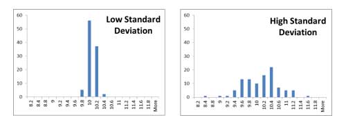
A low standard deviation indicates that the values tend to be close to the sample mean, while a high standard deviation indicates that the values are spread out over a wider range.

Sigma-hat is the symbol used to represent an estimation of the sample standard deviation. More on that later. But the bottom line is that sigma and sigma-hat are similar measures of the dispersion in a data set, and in a perfect world, these two values are equal.
So, the first answer to our question, “What’s the difference between Cpk and Ppk?”, is:
The two indices use slightly different measures of dispersion. Pp and Ppk use the sample standard deviation; Cp and Cpk use an estimation of it.
If my interviewee would have offered this answer, I would have continued listening intently.
To dig a little deeper into this question, we need to consider the origin of the data we’re using to calculate these indices, as the origin of the data determines whether we calculate sigma or sigma-hat.
In one common scenario of measuring process capability, we’re presented with a large batch of parts – say 2,000 pieces – and from that batch, we randomly pull a sample, say 125 pcs. We subject those 125 pieces to a uniform measurement method through which we generate 125 data points – one for each measured value of a given characteristic such as its length or diameter. We then plop those 125 points into our favorite spreadsheet and calculate sigma using the formula shown above. From there, our calculations of Pp and Ppk follow naturally.
In a different scenario, we may want to calculate the capability of an existing process using data from a control chart. A typical variable data control chart plots the arithmetic mean and range of a subgroup of samples drawn at periodic intervals. For instance, you may be responsible for monitoring the cut length of aluminum profiles in an extrusion process that yields 200 pieces per hour. Each hour, the line operator draws 5 samples (referred to as a subgroup), and measures the length of each. She then calculates the x-bar (aka arithmetic average) and range (max x minus min x) of the values in the subgroup, and plots them on a control chart. The notable benefit of a control chart is its graphical depiction of a process’s variation and shifts over time. But we can also use the range (R) data points from our chart to calculate sigma-hat, our estimated standard deviation.
R by itself is an estimation of the process range. The max point in a set minus the min point in a set depicts exactly that, the range of the data. But the R value obtained from a sample has a critical limitation in predicting the process range of a population: its dependence on the subgroup size. In our aluminum extrusion example, each hour the line operator pulls 5 samples to measure. Her R is based on those 5 samples. It stands to reason that if she pulls 10 samples or 50 samples, her R value would more accurately predict the spread of data within the population. Ultimately, if she measures all the parts in a process, her measure of dispersion would be perfectly accurate. Of course, an R based on 2 samples would do a poorer job of estimating the population dispersion. So R2, R5, R10 and R20 are all estimates of dispersion, but useful to varying degrees. The challenge is to measure dispersion (and the resulting process capability) with a useable degree of accuracy, but by using simple tools on the shop floor.
In the 1920’s, Walter Shewhart and his team of engineers at Bell Laboratories solved this problem by developing the Table of Control Chart Constants. One of these constants, d2, was designed to convert the R values collected from a process into an estimate of sample standard deviation regardless of the subgroup size. Here’s the formula Shewhart developed:

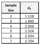
where is the arithmetic average of the individual R’s collected over the course of the process, and d2 is a constant for a given subgroup size. This table shows the d2 values for common subgroup sizes:

Notice as the sample size gets larger, d2 gets larger as well to adjust for its improved predictive value.
Once we’ve calculated sigma-hat, we can feed it into our formulas to calculate Cp and Cpk. Hence, the second answer to our question, ““What’s the difference between Cpk and Ppk?”:
Cpk and Cp are calculated from control chart data, and Ppk and Pp are calculated from batch data without regard to subgroup size.
From where does the idea that Cpk is a measure of short-term capability and Ppk a measure of long-term capability come? The answer: It’s usually a regurgitated sound bite. But there is a bit of truth in this idea, albeit incomplete. Armed with our knowledge of capability analysis, let’s look at this idea more closely.
As we’ve already discussed, Pp and Ppk are calculated by measuring a sample of parts drawn from a larger population. Back to our aluminum extrusion example, if our process produces 200 parts per hour, in 10 hours we’ll have 2000 pieces. By randomly drawing 125 pieces from the 2,000-piece batch, our resulting Pp and Ppk will represent the capability of that entire 10 hours period.
If instead we decide to use our control chart to derive Cp and Cpk, the measure of dispersion driving these indices is , the arithmetic average of the individual ranges of each hourly subgroup. Naturally we would expect R to vary from one subgroup to the next … some larger and some smaller. then is the expected range of any given subgroup.
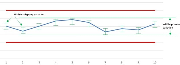
But consider a scenario where the process mean gradually shifts higher and lower over a longer period of time because of some underlying common cause. The range of any given subgroup (a short period of time) would remain the same, but the total range of the process (a longer period of time) would grow in size as a result of the process mean shifting around.

In that case, sigma-hat which uses only the within subgroup variation, would tend to underestimate the population variation as compared to sigma, which uses the entire process variation including both the variation within subgroups and the shifts and drifts between them.
This of course summarizes our third answer to the question, “What’s the difference between Cpk and Ppk?”:
In most cases, Cp and Cpk tend toward a shorter time frame since they consider only within subgroup variation. Pp and Ppk tend toward a longer time frame since they consider the variation that occurs over the entire process study.
So the next time you’re asked that sticky question, “What’s the difference between Cpk and Ppk?”, don’t fear or fall apart. Delivering a clear and convincing answer may just open that next door in your career.
Footnote:
- This article uses the conventions sigma and sigma-hat to represent an estimation of the standard deviation and the sample standard deviation, respectively. Other texts use sigma to represent the population standard deviation, and s to represent the sample standard deviation. Regardless of the convention used, the method is effective is measuring process capability.

